Inspect performances
Sofa provides two ways of monitoring the computation time, one with a text output, the other one with a graphical output.
Command-line method: Advanced Timer
This is the most precise and flexible way of monitoring the computation time in SOFA. It prints results on the standard text output. This can be controlled in runSofa using the following command line options (use --help for the full list) :
--computationTimeSampling arg
-b [ --computationTimeAtBegin ] [=arg(=1)] (=0)
-o [ --computationTimeOutputType ] arg
To monitor the time spent in a specific part of the code, bracket it as shown below:
sofa::helper::AdvancedTimer::stepBegin("Build linear equation");
 // your code here
sofa::helper::AdvancedTimer::stepEnd("Build linear equation");
That is all. Then the corresponding computation time can be displayed at regular intervals. Be careful to use the same string in the two instructions. The begin/end calls can be nested, to monitor hierarchically. An example of statistics is shown below. The number of dots before the name of the piece of code denotes the nesting level.
==== Animate ====

Trace of last iteration :
  *    0.06 ms > begin Mechanical on Cube grid
  *    0.10 ms   > begin Build linear equation
  *                > begin forces in the right-hand term
  *    1.27 ms     < end   forces in the right-hand term
  *    1.37 ms     > begin shift and project independent states
  *    1.49 ms     < end   shift and project independent states
  *                > begin local M
  *    2.11 ms     < end   local M
  *    2.38 ms     > begin J products
  *   12.89 ms     < end   J products
  *   12.91 ms     > begin J products
  *   28.06 ms     < end   J products
  *                > begin local K
  *   28.51 ms     < end   local K
  *   28.53 ms     > begin JMJt, JKJt, JCJt
  *   86.86 ms     < end   JMJt, JKJt, JCJt
  *                > begin implicit equation: scaling and sum of matrices, update right-hand term
  *   87.75 ms     < end   implicit equation: scaling and sum of matrices, update right-hand term
  *              < end   Build linear equation
  *              > begin Solve linear equation
  *   90.78 ms   < end   Solve linear equation
  *   94.81 ms < end   Mechanical on Cube grid
  *   94.83 ms > begin UpdateMapping
  *              - step  UpdateMappingEndEvent
  *   94.84 ms < end   UpdateMapping
  *            > begin UpdateBBox
  *   94.93 ms < end   UpdateBBox
  *   94.94 ms END

Steps Duration Statistics (in ms) :
 LEVEL   START    NUM      MIN     MAX   MEAN     DEV    TOTAL  PERCENT ID
   0       0     100      86.57  127.50  109.99    7.77 10999.1  100    TOTAL
   1       0.06    1      86.32  127.25  109.75    7.75  109.75   99.78 .Mechanical
   2       0.09    1      79.42  112.21   99.97    7.02   99.97   90.89 ..Build linear equation
   3       0.09    1       0.84    1.36    1.14    0.14    1.14    1.04 ...forces in the right-hand term
   3       1.34    1       0.07    0.14    0.10    0.02    0.10    0.09 ...shift and project independent states
   3       1.44    1       0.39    0.68    0.55    0.08    0.55    0.50 ...local M
   3       2.23    2       7.52   17.67   12.72    2.34   25.44   23.13 ...J products
   3      27.70    1       0.28    0.54    0.41    0.06    0.41    0.37 ...local K
   3      28.13    1      54.07   79.54   70.61    5.53   70.61   64.20 ...JMJt, JKJt, JCJt
   3      98.75    1       0.88    2.29    1.31    0.24    1.32    1.20 ...implicit equation: scaling and sum of matrices, update right-hand term
   2     100.06    1       2.71    4.79    3.75    0.51    3.75    3.41 ..Solve linear equation
   1     109.84    1       0.01    0.02    0.02    0       0.02    0.01 .UpdateMapping
   2     109.84    1       0       0       0       0       0       0    ..UpdateMappingEndEvent
   1     109.85    1       0.09    0.28    0.14    0.03    0.14    0.12 .UpdateBBox

==== END ====
In the first line of this table, mean values over 100 iterations of simulation are given. Only the TOTAL value on the first line is the total amount of time elapsed in milliseconds over these 100 iterations. The rest of the table is mean values for each computation step within one simulation step. NUM is the number of times the operation is done per simulation step. It can be noted that "Mechanical" and "UpdateBBox" are the 2 main operations of a simulation step, and the sum of percentages is 100%.
Graphical Interface: Profiler
A graphic tool has been added in order to benefit from a profiling window based on the AdvanceTimer records. This profiler is activated by ticking the box "Display AdvancedTimer Profiler" in the "Stats" widget in runSofa.
This tool is based on Qt5Charts. If this option is grayed in the runSofa GUI, make sure you have the Qt5Charts library and that you properly filled the associated CMake variable Qt5Charts
This option allows to see the animation step duration (ms) in a graphView, then allows to navigate on the graph or on the sliders and analyze the different substeps executed during this animation step. Substeps are displayed in a Tree, in the right order and with their respective time and percentage (with regard to the full step duration). In its design, this tool is inspired from Unity3D profiler.
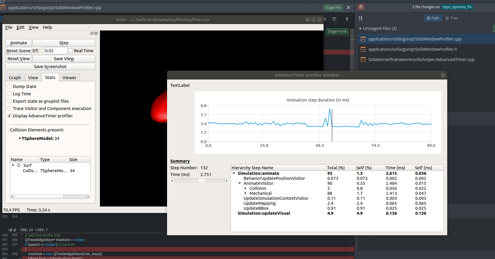
Description of the columns:
- Total (%): Percentage of duration of this step compared to the duration of the root step.
- Self (%):
- If the step has child steps: percentage of the duration of this step minus the sum of durations of its children, compared to the duration of the root step.
- If the step has no child step: percentage of the average duration of this step in case of multiple calls of this step during this time step, compared to the duration of the root step.
- Time (ms): Duration in milliseconds of this step.
- Self (ms):
- If the step has child steps: duration in milliseconds of this step minus the sum of durations of its children.
- If the step has no child step: average duration in milliseconds of this step in case of multiple calls of this step during this time step.
Graphical Interface: Trace Visitor
A graphic tool using Qt exists, and is integrated inside the SOFA main application to trace and profile the execution of the visitors in SOFA. It is work in progress and less accurate than the previous method. It can be used for illustration. How to use the graphic trace of visitors
How to enable the trace of the visitors
You need to activate the option SOFA_DUMP_VISITOR_INFO in your SOFA
configuration. It should be enabled by default. If not, you can use
SofaVerification to modify the configuration of SOFA.
 {.aligncenter
.size-full .wp-image-1293 width="600"
height="342"}
{.aligncenter
.size-full .wp-image-1293 width="600"
height="342"}
Quickly find information
To find a specific visitor, or a call to a component, you can use the
search bar:
 {.aligncenter
.size-full .wp-image-1294 width="600"
height="343"}
{.aligncenter
.size-full .wp-image-1294 width="600"
height="343"}
View State vectors
Another interesting feature is the possibility to trace the evolution
of the state vectors: Just enable the option, and specify the number of
particles; -1 meaning all the particles.
 {.aligncenter
.size-full .wp-image-1295 width="600"
height="343"}
Here, we trace the particles number 2 and 3. A FixedConstraint acts in
this scene on the particle 3: it filters its velocity and acceleration,
and set it to zero, to act as a fixed particle. We can visualize the
effect of the ApplyConstraint visitor on the state vector.
{.aligncenter
.size-full .wp-image-1295 width="600"
height="343"}
Here, we trace the particles number 2 and 3. A FixedConstraint acts in
this scene on the particle 3: it filters its velocity and acceleration,
and set it to zero, to act as a fixed particle. We can visualize the
effect of the ApplyConstraint visitor on the state vector.
Add new debug information
- Trace specific part of the code
To trace and profile the execution of a part of your program, put, at the beginning of the code to profile:
simulation::Visitor::printNode("NameMethod");
and at end the process
simulation::Visitor::printCloseNode("NameMethod");
The method printNode can take other arguments to get a more detailed log;
sofa::simulation::Visitor::TRACE_ARGUMENT arg;
arg.push_back(std::make_pair("ArgumentName", "Value"));
sofa::simulation::Visitor::printNode("MyDebug", arg);
//....
sofa::simulation::Visitor::printCloseNode("MyDebug");
- Trace an additional state vector
At any time in your code, you can monitor a state vector of a given mechanical state writing:
if (sofa::simulation::Visitor::IsExportStateVectorEnabled())
{
   sofa::simulation::Visitor::printNode("MyDebug");
   sofa::simulation::Visitor::printVector(mstate, id); //mstate is a ptr to a mechanical state, id is a VecId, indicating the state vector
   sofa::simulation::Visitor::printCloseNode("MyDebug");
}